This step is generally
called `Cat-A pixel calibration` or `DC to pe`` conversion. In LST the estimation
of the calibration coefficients is performed offline
with so called `F-factor` (or `photon statistics`) method [5], which
permits to estimate the coefficients dc_to_pe in eq. (1).
This method is however affected by some systematic deviations that must be estimated and
corrected. In the next sections we briefly describe the methods, see [3] for more details.
This method permits to estimate the effective gain of the pixels, defined as gain = 1/ dc_to_pe.
It makes use of the statistical correlation between the charge dispersion of a signal
and the number of photo-electrons (\({N_{pe}}\)) originally produced by the light
in the photo-cathode.
In fact, in the case of an ideal poissonian detector, the integrated charge \({Q}\)
produced by an incident light pulse on a PMT and its standard deviation, \({\sigma_{Q}}\) (when repeated several times)
are related to the gain (g) by the following simple relations:
(3)#\[\begin{eqnarray}
g & = & \frac{\sigma_{Q}^{2}}{Q}
\end{eqnarray}\]
For a real detector the relation is more complicated due to added noise components.
In particular, for LST, where \({Q}\) is produced by flat-field events, the
variance \({\sigma_{Q}^2}\) is given by:
where \(Q_{ped}\) is the pedestal charge, \(\sigma_{Q_{ped}}^2\) is its variance,
\(F = \sqrt{1 + \sigma_{spe}}\) is called `excess noise factor`
and depends on \(\sigma_{spe}\), which is the single photon electron width in pe, B is
a quadratic noise term due to the DRS4 time sampling irregularity and the intrinsic
pulse light dispersion of the laser (see [3] for more details).
Hence, the formula used to estimate the gain in LST is :
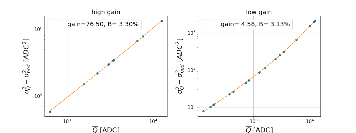
The systematic term B in eq. (4) is estimated, per pixel, by the fit of the
charge variance of an intensity scan obtained by changing the Calibox filters in front of the laser.
Example of intensity scan fit, based on eq. (4), for both channels of one pixel.#
In short:
Input data : flat-field and NSB pedestal events from an intensity scan
This calibration is performed in order to improve the Cat-A calibration (based on fixed coefficients for the full night)
with a continuous estimation of the camera gain during the night based on interleaved calibration events.
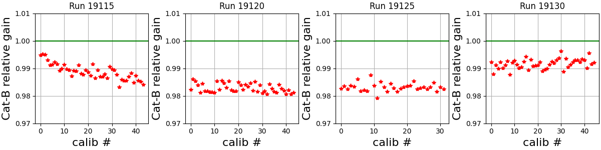
In this case, the F-factor method is applied to calibrated waveforms, the estimated Cat-B gain is then relative
to the Cat-A gain. Therefore, if no changes are present during the night, the Cat-B gain is expected to be
one. In general, smooth changes of less then 2% are observed.
Example of Cat-B gain estimation for some runs of a night.#
In short:
Input data : interleaved (calibrated) flat-field and NSB pedestals events